For a given proportional load, the software determines the load level for which the first ply failure occurs. The software also makes possible to determine the failure envelope of the multi-layered material with the FPF (first ply failure) criterion.

The mechanical loads considered by the software are generalized loads. In this way, we may apply to the multi-layered material:

• A membranar force N_x or a generalized strain e_xx
• A membranar force N_y or a generalized strain e_yy
• A membranar force N_xy or a generalized strain e_xy
• A moment M_x or a generalized curvaturec_xx
• A moment M_y or a generalized curvature c_yy
• A moment M_xy or a generalized curvature c_xy

The software also lets to take into account residual hygrothermal strains. MAC LAM predicts the load level that may cause the first failure in a layer (FPF criterion). In order to predict the limit for a layer failure, the software calculates the stresses (with the help of a classical laminate model [1] ) within the layer in the local coordinates system and uses the failure criterion of the layer. This failure criterion may be selected among the criteria programmed in MAC LAM. These criteria are:

• Tsai-Hill criterion

(1)

• Hoffman criterion

(2)

• Tsai-Wu criterion

(3)

where , , , , , F₁₂ is a constant that has to be defined by the user; X_t, X_c, Y_t, Y_c and S are the material strengths defined in [1].

The generalized loads that may be applied to a multi-layered material define a six-dimensional space: e.g. the space (N_x, N_y, e_xy, c_xx, M_y, M_xy). The failure envelope in this six-dimensional space is supposed to be convex.

Figura 0. Intersection of the failure envelope with a 2D plane

MAC LAM makes possible to visualize this failure envelope by means of two kinds of calculations:

1. In the first one, the user defines a load direction. For instance, the vector

defines a load direction. MAC LAM next determines, assuming a proportional load in the load direction, the factor times which the vector has to be multiplied to be in the failure limit of the weakest layer. MAC LAM determines in this way the intersection of the given direction in the six-dimensional space with the failure envelope (which is, as matter of fact, a hypersurface). MAC LAM also gives the number(s) of the weakest layer(s), the contributions to the failure criterion of every term of the criterion.

2. In the second one, the user may visualize in a two-dimensional space the failure envelope of the six-dimensional space. To do this, the user defines a plane defined by two dimensions (for example; N_x and N_y) and by the plane position in the six-dimensional space. This position is given by the definition of intersection of the plane with the axes corresponding to the four remaining dimensions (for example (e_xy = 0, c_xx = 0.00001, M_y = 0, M_xy = 0.001). The result of this type of calculation provides the intersection of the plane previously defined with the failure envelope.

Now we will see in a more detailed way how to operate MAC LAM in order to get these results:

• In first place, it is necessary to define the laminate paying attention when filling the columns (in the multi-layered material table) which contains the layers failure criterion data (do not forget that for Tsai-Hill, Hoffman and Tsai-Wu criteria, we have to write 1, 2, and 3, respectively in the column <<Criterion>>)
• then you have to define the visualization method for the failure envelope
• after that, the Calculation and report options have to be selected
• then you have to click on the button <<Analyze>> in the main window (see Figure 1)

Figure 1. Launching STRENGTHS calculations.

What follows depends on the selected visualization method:

• You selected the first visualization method: to look for a point in the failure envelope for a proportional load
• You selected the second visualization method: to plot the intersection of the failure envelope with a plane
  

Results of the first visualization method (intersection point)

If you selected the first visualization method (to look for a point in the failure envelope for a proportional load), you will see appear a new window similar to that in Figure 2. In this window, the graph represents the contributions of the criterion terms in the total value of the failure criterion (the column on the right side) and this, for the layer under consideration. If total value is 1, the layer under consideration is the weakest one (the one which will fail the first). In order to achieve a better understanding of this, let us describe the meaning of results in Figure 2.

Figure 2. Window of results in the first visualization method.

The graph in Figure 2 corresponds to the first layer in the stacking sequence. For this layer, the criterion selected was the Tsai-Hill criterion. This criterion was calculated based at the lower boundary of the layer. The Tsai-Hill criterion has four terms (cf. Equation (1)):

1. The first one is
2. The second one is
3. The third one is
4. The fourth one is

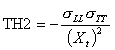
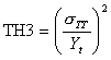
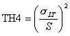
If the Hoffman, or the Tsai-Wu criterion were selected, the terms would have been (H1, H2, H3, H4, H5, H6) or (TW1, TW2, TW3, TW4, TW5, TW6) respectively. In the corresponding criterion, each one of these terms corresponds to a term in the equation in the order they occur.

Let's get back to the case in our example: we selected the Tsai-Hill criterion for the first layer. To every term corresponds a column of the graph in the Figure: the last column is the sum of all of the terms (TOTAL). In the graph, we see that the TOTAL is approximately 0.2 (<1, so there is no failure in the first layer at its lower bound) and it is the first term the one which contributes the most to this total.

In the lower part of the window, you may look for the point of intersection with the failure envelope and the number of the weakest layer (see Figure 3). You may also visualize the results for another layer and on another position in the layer by clicking on the options located in the lower left part of the window (see Figure 3).

Figure 3. Change of layer number and position.

So as to change the colors of the chart, click on the button <<Chart options>>, and to create a report that you can print with all of the results, click on the button <<Create a report>> (see Figure 4).

Figure 4. Chart options and creation of a report.

Results of the second visualization method (2D shear)

If you selected the second visualization method (to plot the intersection of the failure envelope with a plane), you will see appear a window similar to the one in Figure 5. The plotted curve represents the intersection of the failure envelope with the plane whose coordinates are those that you defined in the option <<How do you want to visualize the failure envelope?>>.

Figure 5. Visualization of the failure envelope.

If you want to view the coordinates of the points of the curve, you have to click on the button <<Point values>> (see Figure 6). You may also look the numbers of the layers that break for every point of the curve by clicking on the button <<# of broken layers>> (see Figure 6).

Figure 6. Visualization of point values and number of broken layers.

You can create a graphical or textual report to print them later by clicking on the buttons in Figure 7. The textual report contains all of the data you selected in <<Options>>. Furthermore, you may save the points values for plotting them with another software like Excel by clicking on <<Save the values in a file>> (see Figure 7).

Figure 7. Reports and saving the values in a file.

Visualization method for the failure envelope

In the main window of the module you may select the visualization method for the failure envelope by clicking on the button in Figure 8.

Figure 8. Visualization method.

Next you will have to select the visualization method in the options in Figure 9.

Figure 9. Selection of the visualization method.

• If you select the first method, you have to define the load direction by choosing the stresses or strains by filling the 6 fields in Figure 10. You can also give (in the lower part of the window) the temperature and moisture variation values in case you decided to take into account the thermal and hygroscopic strains in <<Calculation and report options>>.

Figure 10. Definition of the load direction for method 1.

• If you select the second method, you have to define the plane by its 2 axes and by its coordinates with the options in Figure 11. You have to define the number of points per quadrant for plotting the failure envelope intersection with the selected plane (you can do it in the left lower part of the window), too. You may also give (in the lower right part of the window) the temperature and moisture variation values in case you decided to take into account the thermal and hygroscopic strains in <<Calculation and report options>>.
  

Figure 11. Definition of the intersection plane for method 2.

Calculation and report options

Before you launch your calculations, you have to define the calculation and report options by clicking on "Options" in the menu bar of the main window in Figure 12.

Figure 12. Go to calculation and report options.

Now the window in Figure 13 appears. It is necessary to specify

• whether you want to take into account a thermal load or not. If this is the case, give the temperature variation value in the visualization method window.
• whether you want to take into account hygroscopic strains or not. If that is the case, give the relative moisture variation in the visualization method window.
• everything you want to have in the textual report.

Figure 13. Calculation and report options.

References

[1] R.M. Jones, "Mechanics of composite materials", second edition, Taylor & Francis, United States, 1999.